Interactive Graph Entropy
This page lets you explore the notion of (conditional) graph entropy through a number of interactive tools. Before you start, you may read this gentle introduction first: PDF.
For more material look at the references at the bottom of this page. In particular, you may read Simonyi's excellent survey [Sim] on graph entropy.
The codes below use this GitHub repository, which contains an implementation of an alternating optimization algorithm for (conditional) graph entropy described in [HNB2].
1. Graph entropy visually
Hit 'Go!' and pick/define your graph G. Then HG(X) is computed via alternating optimization. The optimal weights (rj) of the independent sets are shown along with a bar chart representing the corresponding optimal point (ax) in the vertex-packing polytope VP(G). If uniform_X is unticked, then the distirubution of X is generated randomly.
2. From empty to complete
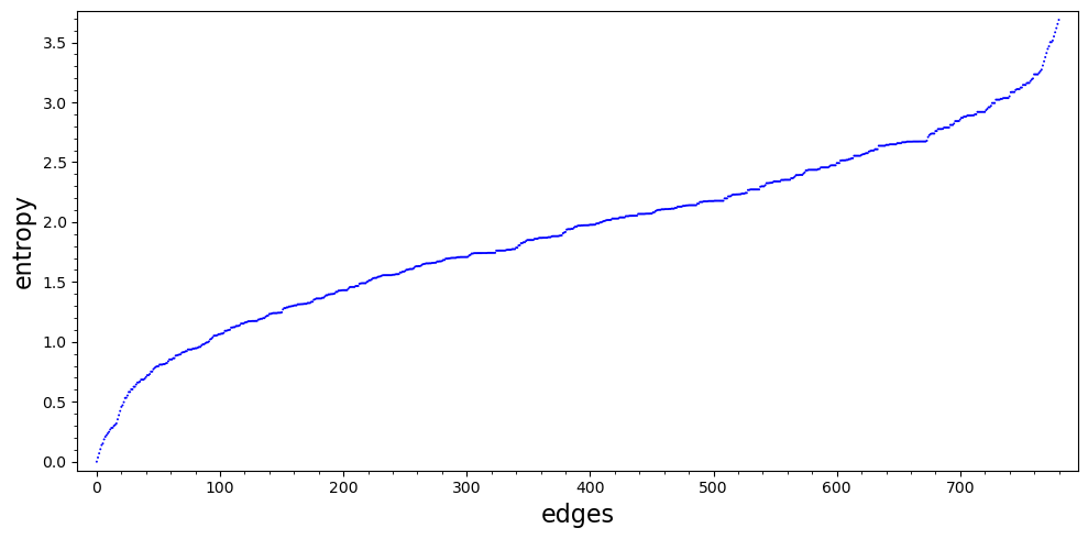
How does graph entropy typically change when moving from the empty graph to the complete graph? We add edges randomly one by one, and plot HG(X) for a uniform $X$ after each step.

40 vertices:

Hit 'Go!' and create your own animation. Define the distribution of X by a list of probabilities and set block to be the number of edges added in one step. (Use larger block to speed up the running time.)
3. Entropy vs edge density
In a similar experiment, the code below allows you to plot graph entropy against edge density. For a complete graph G on N vertices we have HG(X)=H(X)=log(N) for uniform X. So it is natural to look at HG(X)/log(N) for various graphs on N vertices and plot it in terms of the edge density of G. Hit 'Go!' and choose your favourite N's! The resulting plots will be displayed separately for each N, as well as in a single figure with different colors representing different values of N.
4. Error bound vs true error
For vertex-transitive graphs we know the true value of graph entropy for uniform X:
So we can track how the error of the iterative algorithm decays (and how it compares to the guaranteed error bound). Hit 'Go!' and pick your favourite transitive graph! The value and the error are computed after every block iterations. Also, you can turn set-deletions on (which should speed up convergence) by setting factor_active to a positive value. The initial weights (i.e., starting r) are generated randomly here.
To track the error for some non-uniform X, let's take a cycle of odd length 2n+1. If X is close to uniform, then the true value of graph entropy can be easily computed. Specifically [HNB2]:
Hit 'Go!' and pick a cycle length.
5. Conditional graph entropy (CGE): Orlitsky–Roche example
In [OR] Orlitsky and Roche condidered the example where G is a graph on three vertices with a single edge, and (X,Y) is uniform random conditioned on X≠Y.
Error. The code below chooses a random starting point r(0) and runs alternating optimization. After each iteration, it prints the current ϕ-value, its distance from the true value HG(X|Y), and the error bound (guaranteed by the dual problem). Hit 'Go!'
Convex corner. Below you can look at the 3D plots of the boundaries of the convex corner Ka (blue) and the (upward-closed) convex set L-1 for the Orlitsky–Roche example. A two-dimensional cross section is also plotted. Hit 'Go!' and use your mouse/touchpad to change the viewpoint for the 3D plot.
Optimal points. The convex corner Ka depends on the graph and on the conditional distributions Y|X=x for each vertex x. So we can fix these as in the Orlitsky–Roche example and vary the distribution of X (described by the probabilities px) in order to get different optimal points a in Ka (they should all lie on the boundary). The code below finds the optimal point a for randomly chosen px, and plots such optimal points along with the boundary of Ka. Hit 'Go!' and press 'Update' to add more points. (You may use your mouse/touchpad to change the viewpoint for the 3D plot. Some of the optimal points may appear to be slightly off the boundary but this is only due to the inaccuracy of surface plotting at places where the z-axis of the surface changes too abruptly.)
6. CGE: random bipartite graph
The code below generates a random bipartite graph with partite classes of size N1 and N2 and with edge probability pr. Then it generates a random probability array px,y of size (nr_x)×(nr_y), where nr_x=N1+N2, and calculates the corresponding conditional graph entropy. Hit 'Go!'
7. CGE: create your own setup
The code below lets you define a graph through its adjacency matrix and set some px,y to zero. Then it uses uniform X, and for each x uniform Y|X=x (among the nonzero values). Then it performs steps iterations of alternating optimization (no set deletions!), printing the current ϕ-value and error bound after each iteration. At the end it prints the final r and the corresponding a. You may change the values of nr_x and nr_y in the code, then hit 'Go!'
8. Write your own code
Before hitting 'Go!', read through the code below. The comments guide you through the different features of the GraphEntopy class. Make some changes in the code and hit 'Go!'
References
[Intro] Introduction to Graph Entropy.
[Sim] Gábor Simonyi Perfect graphs and graph entropy. An updated survey. In Jorge Ramirez-Alfonsin and Bruce Reed, editors, Perfect Graphs, pages 293–328. John Wiley and Sons, 2001.
[CsKLMS] Imre Csiszár, János Körner, László Lovász, Katalin Marton, Gábor Simonyi Entropy splitting for antiblocking corners and perfect graphs Combinatorica, 10(1):27–40, 1990.
[OR] Alon Orlitsky, James R. Roche Coding for computing IEEE Transactions on Information Theory, 47:903–917, 1998.
[HNB2] Viktor Harangi, Xueyan Niu, Bo Bai Conditional graph entropy as an alternating minimization problem to appear in IEEE Transactions on Information Theory.
[HNB1] Viktor Harangi, Xueyan Niu, Bo Bai Generalizing Körner's graph entropy to graphons to appear in European Journal of Combinatorics.